TI BAII Plus Calculator Advanced Functions for the CFA® Exam

- Capital Budgeting
- Uneven Cash Flows
- Mean, Variance, and Standard Deviation
- Covariance, Correlation, and Regression
- Depreciation
How To Use Advanced TI BAII Plus Calculator Functions for the CFA Exam
In this volume in the Schweser Video Library, we want to talk about some of the more advanced features and functions on the Texas Instruments Calculator.
Sign up for our CFA question of the day and get a CFA question sent directly to your inbox every day to help prepare for the next sitting.
Video Transcription
Things we’ll cover here have to do with capital budgeting. First off, that’s probably the most important here, and then we’ll show how you can use those cash flow keys to do uneven cash flow calculations, either present value or future values on those. Then we’ve got some statistical functions here…mean, variance, and standard deviation, covariance, correlation, and regression. And then finally, a couple of depreciation, straight-line, and accelerated depreciation methods.
Capital Budgeting with TI BAII Plus
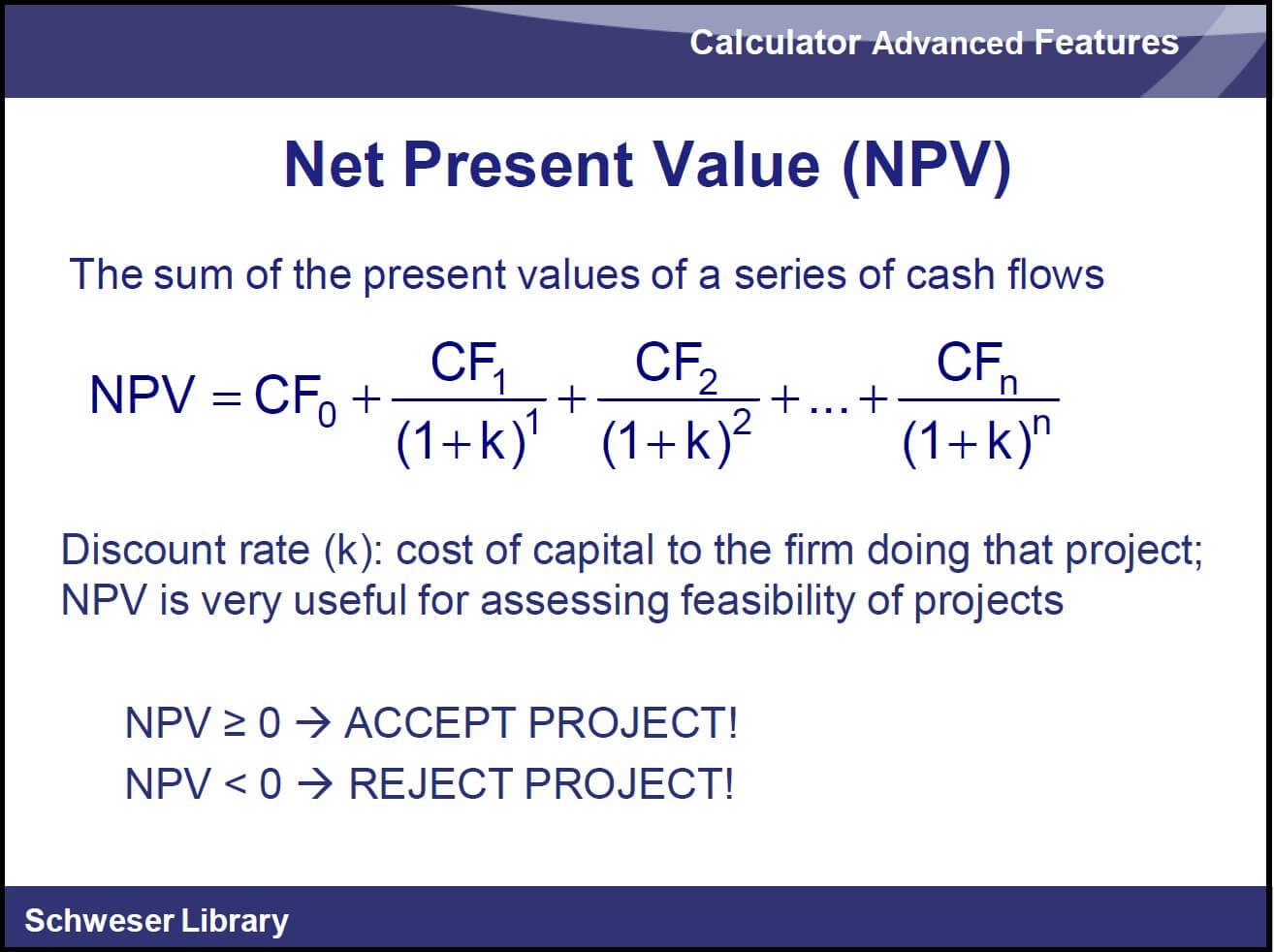
So let’s start off with capital budgeting first. The idea of capital budgeting is we’re going to make an expenditure today. And then we’re going to get returns from that over a number of periods in the future.

In the basic calculator video, we talked about using the time value of money keys. There we had a payment, but it had to be the same payment every period. So we need to enter these expected cash flows. So here’s our initial outlay. That’s going to be CF0. We’ve got to enter that as negative. Then this will be our cash flow 1 here. And this is cash flow CF2, CF3, and CF4.
Now, one thing about entering these cash flow keys is we’re going to tell it how many of these in a row there are. So here, we’re going to have to enter in 1, 2, 3, and 4 because they’re all different. Let me just clear this off and give you an example.
Say that this cash flow was $100 instead of $75. So this would be cash flow 1, and this would be cash flow 2. And then we’d say the frequency of cash flow 2 is 2 because there’s 2 of these $100 payments in a row. And this would actually be cash flow 3 because that’s the third different cash flow out here beyond CF0, our -175.
So, clearing this off, we’ll see we’ve got four to enter, so let’s go through that entering procedure.


We had a positive Net Present Value at a discount rate of 10%. So clearly, in order to get to a zero Net Present Value, we’re going to have to increase that. Our internal rate of return should be higher than that 10% because we had a positive Net Present Value when we use 10%.

So, same cash flows we want to use. Initial outlay 175 and positive cash flows after that 25, 175, and 50.

As far as entering those, this is exactly the same as what I showed you before. As a matter of fact, if you put those in, you don’t have to do this again because those cash flows are already entered in there. In that case, you can just press the IRR key.

Once you’re in that cash flow mode, press the IRR key and then COMPUTE and find out that the internal rate of return here is 15.067%.
Now, another calculation that we can do here is the Payback Period and Discounted Payback Period. This is a measure of liquidity…how long does it take to get back the initial investment?
So it’s not a measure of value. It ignores the time value of money, and it ignores any cash flows beyond however many years it takes to get the original investment paid back.

So, what we want to do here conceptually is say, “With Payback Period, how long does it take to get back $175?” If we get back 25 there, we have to get back 150. If we get back 100 there, we’ve got 50 to go. And since there’s 75 in this third period, we need 50 of that, which is two-thirds. So we’re expecting to get something like 2.67 as our Payback Period.

So, let’s enter all these cash flows. This is the same as we did before. We’re still using the cash flow keys.
So we enter all those single cash flows, go into Net Present Value. Tell it the discount rate is 10, enter that 10, scroll down, and get to NPV.

Then we can also get to NFV, Net Future Value, and then finally to the Payback Period.
Once we get to the Payback Period, if you want to compute that, press COMPUTE, and it will tell you it’s 2.67 years, as we suspected.
The Discounted Payback Period is how long it takes to get your original investment back in present value dollars, in discounted future cash flow dollars. So that’s going to be longer than two and two-thirds of the year.
Go to scroll down with the arrow key until you see Discounted Payback. That will be the next one, in fact. Press COMPUTE and find out that that is 3.39 years. So again, once you’ve got the cash flows in, you really can’t go too far wrong here on calculating these.

Another measure from corporate finance that we might want to calculate is the Breakeven Quantity of Sales. This just says how many units you have to sell to just cover your fixed costs.
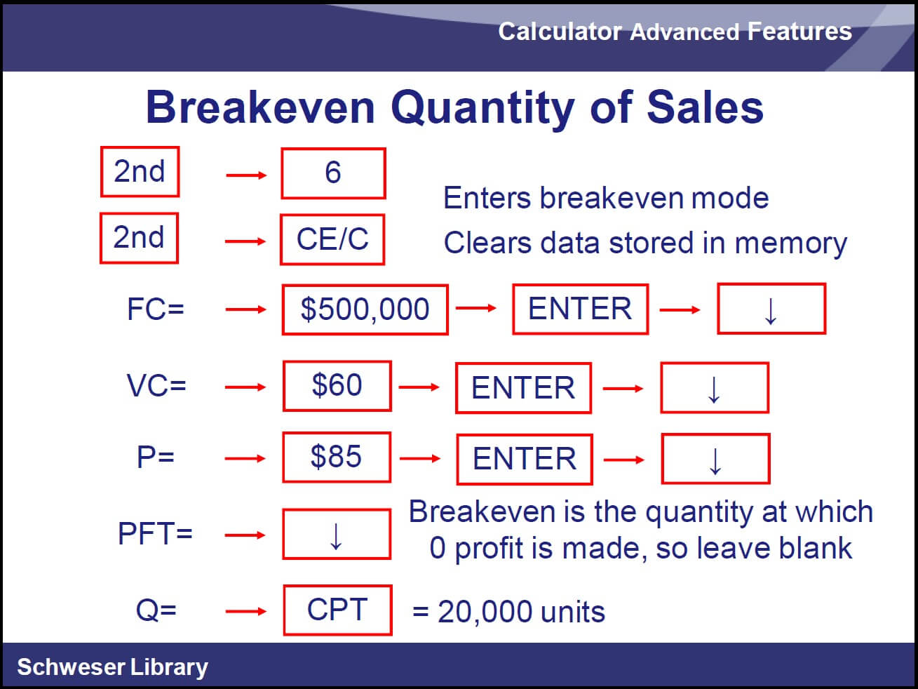
So if you use the second key and then hit 6, that gets you into the breakeven mode. Clear all the entries in there.
First off, put in your fixed costs and don’t forget to hit ENTER. Put in your variable cost per unit. This is a total fixed cost, and this is variable cost per unit of $60. We said that the price will be 85, so enter that and then scroll down. You get the profit. We’ll scroll by that. Since we’re not using it right now, scroll down to quantity and COMPUTE and get 20,000 units.
That says, in order to just break even on an operating basis, we need to sell 20,000 units. That $25-unit difference between the price and the variable cost…that’s what goes to cover fixed costs. And at 20,000 units, we just generate the $500,000 necessary to cover our total fixed cost.
Calculating Uneven Cash Flows with TI BAII Plus
Now, we can use this for some uneven cash flows. Remember with our time value of money keys, we had to have equal payments every period. What if we got to a situation where we said, “Well, there’s some uneven cash flows.”

Here’s what we expect to receive at the end of each in the next three years or at the end of this year and each of the next two years. Time 3, three years from now, it’s the end of the second or third year; however, you want to count them. But we’ve got payments at the end of the first period, the end of the second period, and the end of the third period.
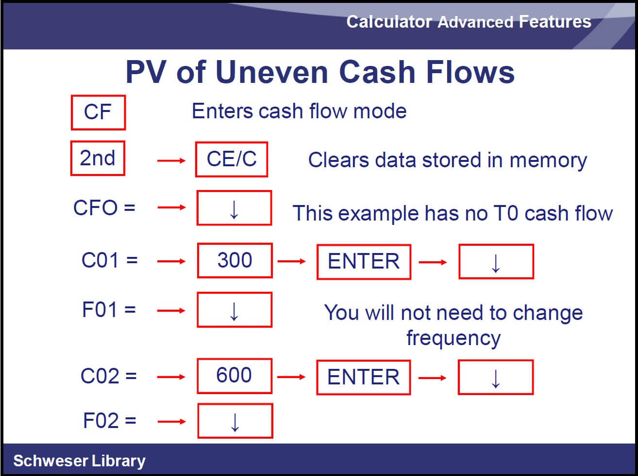
So, we’re in end mode here, and we’re going to put those cash flows in just like we did for Net Present Value, except we’re going to leave CF0 at zero. Remember that Net Present Value function takes the present value of all those future cash flows and subtracts off CF0, our initial outlay. Actually, it adds to it.
That’s why we enter it as negative. But if we just put that in as zero, then it’s subtracting off zero, and we’ll get the present value of all those future cash flows.
So again, we’ll enter 300 with a frequency of 1. So we can scroll by that. We’ll enter 600, which also has a frequency of 1. So we can scroll by the FO2, which is already set to one.

We’ll enter that third cash flow and then enter the NPV, Net Present Value mode. Tell it that the interest rate is 10% again, hit ENTER, and scroll down, and then we get our Net Present Value. We’ve got to make it compute that, so we press COMPUTE, and we find out that the present value of those three cash flows is 9, 18, 86.
So it was no different from Net Present Value except we put in zero for that initial cash flow. So nothing was subtracted off of that present value of those three future cash flows.
Future value of uneven cash flows, we’re just going to scroll down to future value and press COMPUTE. But I think you need to understand what we’ve got here. If we put $300 into a bank account that earned 10% compounded annually, after two years that time 3 here, the end of the third year, 300 would have grown to this amount here.
The 600 grows for 10% for one period, so that’s going to be turning into 1, 6, or 660 one year out. And then we just add all these up to get the future value. So, if we’re making these deposits into the account of 300, 600, and 200, and it was earning an annual compound rate of 10%, at the end of that third year, right after we put in that last $200 deposit, the future value is what we would have in the account.
So again, the entry of this is exactly the same, and if you did it before, they’re already entered in your calculator.

So now go to Net Present Value mode. Tell it it’s 10. If you put that in before, it already knows that. So scroll down from Net Present Value to Net Future Value, then hit the COMPUTE key and find out that that amount we’d have at the end of the third year, end of year 3, $1223. Now, that Net Future Value, it’s only on the professional edition here. It’s not on the plastic one.
Learn How to Use a Mock CFA Exam to Sharpen Your Testing Skills
Calculating Mean, Variance, and Standard Deviation with TI BAII Plus
So now let’s take it to look at some data entry and some statistical functions.

We want to look at the population mean and the sample mean, which are the same. It’s just the simple average of the values from our sample.

And so our population and sample mean, let’s say we’ve got three years with the data, six, and eight, and a four. We can pretty much do this in our head. But for more complex problems, you may want to use the calculator.
So calculate the mean return. We know it’s 6 because 6 plus 8 plus 4 is 18, divided by 3 equals 6.

So how do we enter these? Second seven gets you into the data entry mode, and it just says data above the seven key. So we’re going to put this in, and first clear everything out and then put our first X variable in as six, hit ENTER and scroll down.
When you scroll down, it’s going to prompt you for Y, 01, the first value of Y. We only have one variable here, and we’ve got historical data. So we’re just going to skip past that. ENTER 8 for the second value of our X variable.

ENTER 4 for the third value of our X variable. Scroll down and then enter the statistics mode, which is that second function on the 8 key.
Now, go to second, ENTER and keep pressing that until 1V appears. That is, we’ve got to tell the calculator, “Hey, we only told you one variable.” And then as you press the down arrow now from 1V, that’s really the set key when we’re doing second ENTER, second ENTER. We’re looking at all those different functions we might use. We get to the one that says single variable analysis. That’s the 1V. Once we get there, no more second function. Hit the down arrow and as that scrolls down, we’ll get the simple average of our three values of X, which is six as we knew.

Now, if we wanted to put probabilities in there…say we had a probability model that said, “If the economy is average, and there’s a 30% of an average economy, return is going to be 6%. If we have a great economy, there’s only a 20% probability of that, but the return would be 8%.
If we have a crummy economy, there’s a 50% chance of that. Our return is going to be 4%.” So this is what I call a probability model, as opposed to just getting historical data from each year, or each quarter, or each month, or whatever it is.
So now, we’re going to enter these as whole numbers, 30%, 20%, and 50%, and calculate the mean return. If it’s a weighted mean return, or the other thing, it’s the expectation of X, the expected value of this.
And so that, from a mathematical standpoint, we’re going to multiply each one times the probability and add them all up. Here’s our calculation here. And we’d take that sum, and that sum would be this weighted mean or expected value.

So, let’s go to our data entry mode again. And when we put in 6 this time, we’re going to put in 30 for Y. It’s not really a Y variable. It’s the probability. We’re going to let it know that that’s a probability by telling it we only have one variable. And it’s going to know, If they only got one variable, these others must be probabilities. Those probabilities also need to add up to 100 so you don’t get an error message.
So, 6 has a probability of 30%, so we ENTER, scroll down. Eight, ENTER, scroll down, 20% probability, ENTER, scroll down.
Four has a 50% probability, ENTER, scroll down twice, and then enter statistics mode. Now, again, we need to tell it that there’s just one variable. And when we do that, it will calculate that weighted average of those three values using those probabilities as weights as 5.4, and that’s 5.4%.

Now, what about our Sample Variance and Sample Standard Deviation? Our calculator will do the Sample Standard Deviation for us. Here, we’re dividing by N minus 1 to calculate the sample variance. And we use the sample variance when we don’t have every outcome in the whole population but just a sample.

So, here we go again, six, eight, and four. We can enter these as decimals or enter them as whole numbers.
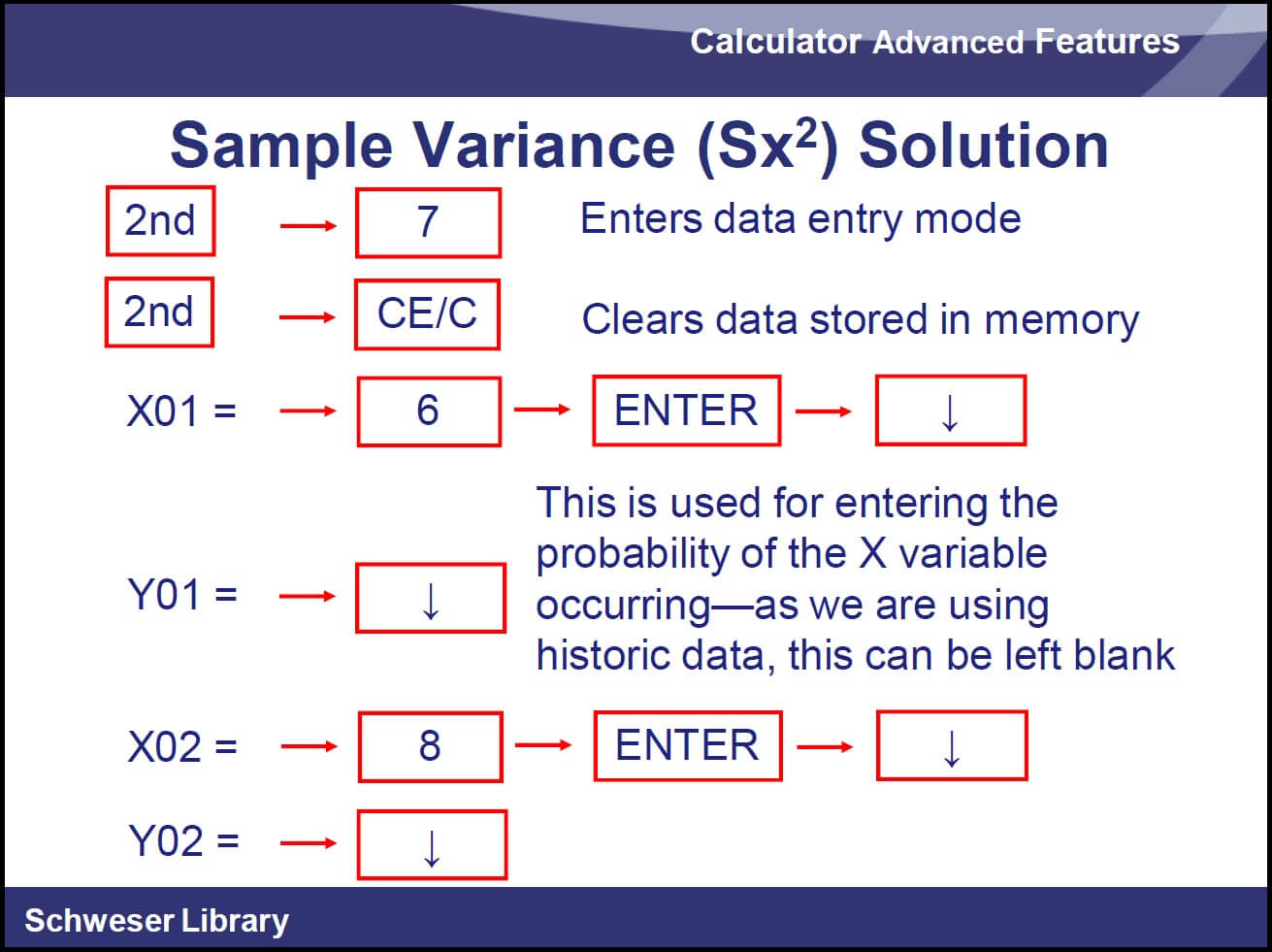
Then we enter data entry mode, clear everything out of the data entry mode, and enter these. Since you already have these in, but you had them in with probabilities, maybe you want to redo it and leave nothing for those probabilities.

So then we go back to statistics mode, tell it it’s a single variable, and get our sample standard deviation of two, and we can square that. So it doesn’t give you the variance. It gives you the Standard Deviation. All you need to do is hit X2 to see what the variance is.
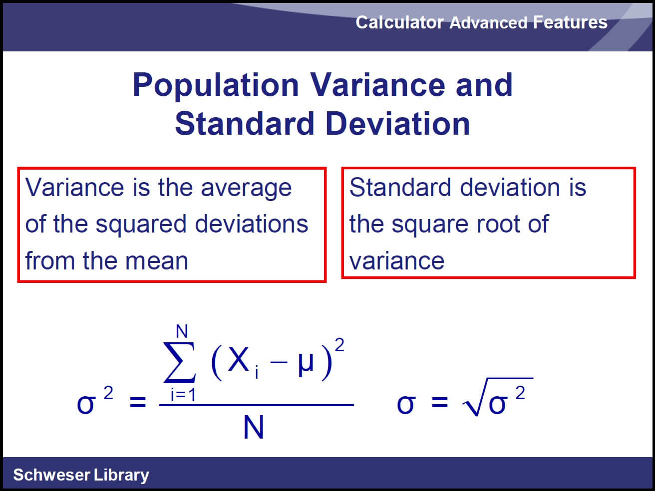
Now, when we want to calculate Population Variance and Standard Deviation, we’re really dividing by N. So notice as you scroll down through these…FX is Sample Standard Deviation. Sigma X, we reserve the Greek letter for the population.
Now, what does it matter to you? If you’ve got a sample, you calculate sample standard deviation. If you have every possible outcome in the whole population, then you divide by N and calculate the Population Standard Deviation and square that to get the variance.

Now, what if we had one of these probability models? We can do that as well. We can enter them the same as we did before.

So we enter those probabilities as the Y’s, right here and right here. We enter the X values as the X’s, and then we tell it it’s one variable.

When we tell it it’s one variable, it knows that those Y values are probabilities. And we can go down and find the Population Standard Deviation, given that the probability model is 1.56%, and then we can square that to get 2.44 for our Population Variance.
Get Access to Free CFA Study Materials
Calculating Covariance, Correlation, and Regression with TI BAII Plus
Now, let’s look at some other statistical functions here…covariance, correlation, and regression.
Now we don’t do any regression at Level I, but you might as well learn it while you’re learning this. We do deal with correlation and covariance.
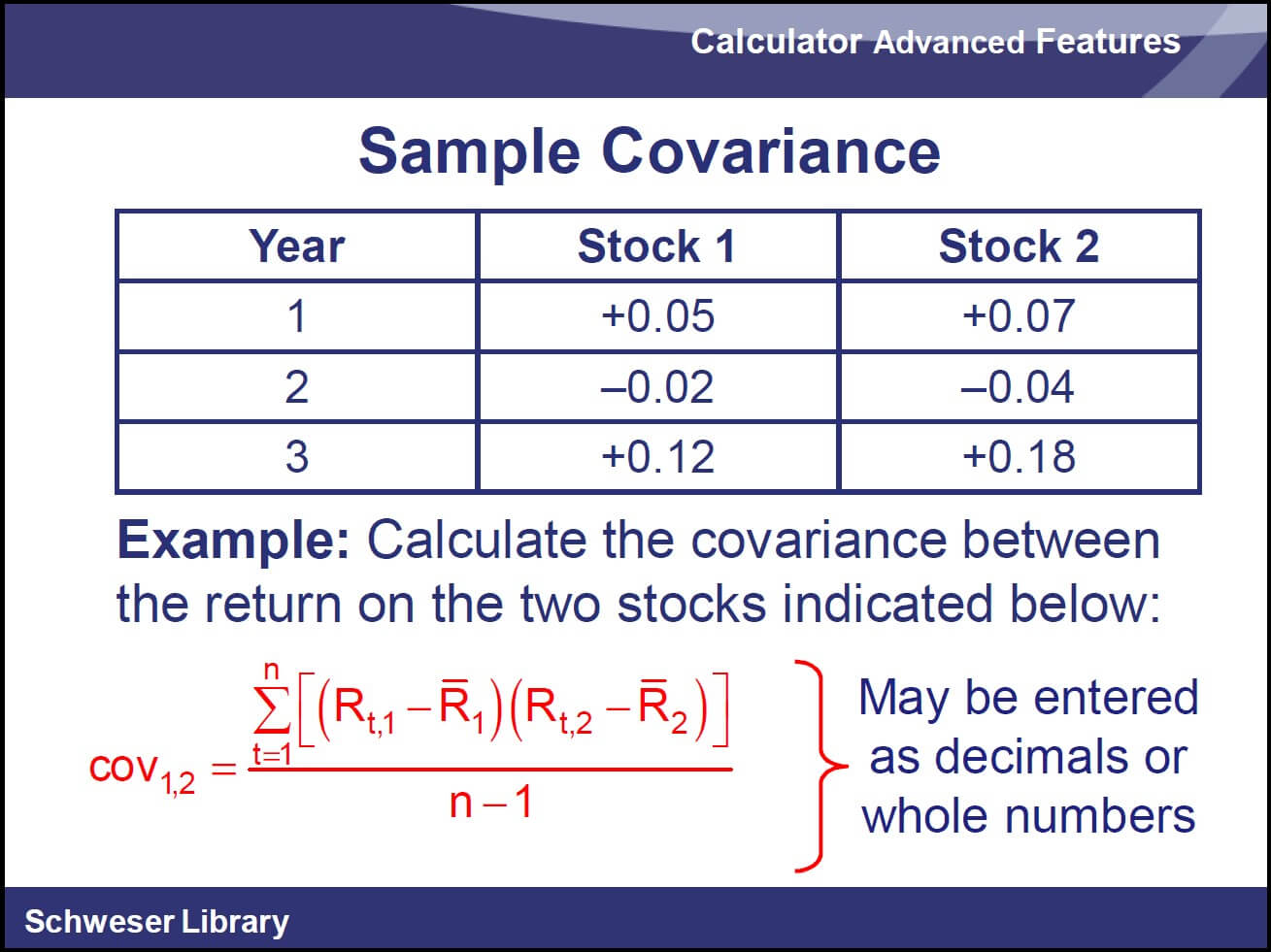
So the idea here is we have three values for each of two variables, but each variable has a value for each period. So, in year 1, Stock 1 was up 5%, and Stock 2 was up 7%. In year 2, -2% of -4%, etc.
The mathematics is covariance. For each of these periods, we’re going to take the difference between…and I guess I could write this as X-bar…the expected value of X. We’ll take the deviation from the mean or the weighted mean.
In this case, just the simple mean and multiply that times the difference over here, taking off the expected value of Y. So we multiply those together. We add them all up for each of the three periods and then, because it’s a sample covariance, we’re going to divide by N minus 1. In our simple example here, N minus 1 is just 2.

So, we enter the two values. Now, we’re going to enter X1 and Y1, the 5 and 7, the -2 and the -4 for X2 and Y2. And in the third period, our values were 12 for X and 18 for Y. So we enter those as well and just keep scrolling down.

Now, we enter statistics mode and use that second set key, which is the second function or the ENTER key, and keep pressing until you get to linear regression. Now as we press the down arrows, it will give us our regression statistics.
So what is N? How many observations did we put in? We put in three. Here’s the mean of X…SX. Remember with the letter S, it’s the sample standard deviation of the X variable.

Keep scrolling down. We’ll get the population standard deviation. That’s using the Greek letter Sigma, lower case Sigma and then the mean value Y, sample standard deviation Y, population standard deviation Y, intercept of our regression line, and gradient of our regression line.
So if we had some data and fit a line that fits the best data, it would give us this point here. That would be our intercept of our best fit line. And the gradient of that is the slope of the line.
We don’t need these for Level I. It’s good to know they’re there. What we need is this correlation coefficient. This calculates the sample correlation between X and Y over the periods that we’ve got.

So, we’ve got the SX is seven. Sample standard deviation of X is seven. Sample standard deviation of Y is 11. We’re given a correlation. We had perfect positive correlation for X and Y and came up with one.
Now, your calculator is not going to tell you the covariance. But the definition of correlation coefficient is covariance over the product of the standard deviations. That’s the correlation coefficient. So in order to calculate the covariance from that, we use this correlation coefficient. Actually, it’s in there as R times the two sample standard deviations.
So that’s what we’re doing here. RCL 1 is our 7, RCL 2 is our 11, and RCL 3 is our correlation coefficient. So here’s what we’re going to do. We’re going to multiply that correlation coefficient times the product of the two sample standard deviations. And that way, we can get to our covariance once we’ve entered our data.

Now, we also need to be able to calculate the covariance and correlation for a joint probability function. But there’s really no calculator function for that, because here we’ve got a probability model, and we’ve got two values for each one. We aren’t really set up to do that on the calculator.
So you’ll have to follow the method that we give you in the SchweserNotes for calculating covariance and correlation from a joint probability function.
As long as we’ve got this in front of us, what it says, there’s a 15% probability that the return on A will be 20%, and the return on B will be 40%. So there’s only three possible outcomes here: 20% and 15%, or 0% return on B, and 4% return on A. There’s a 25% probability of that outcome. So no real shortcut using the calculator on that one.
Calculating Depreciation on TI BAII Plus
Let’s take a look at some depreciation measures here to wrap things up.

For straight-line depreciation, it’s just the original cost minus the salvage value over its depreciable life. So this is not a difficult calculation for straight-line depreciation expense.

But there is a depreciation function, a depreciation mode on your calculator. It’s the second function above the four key. Clear everything out of there using second; and you clear entry and then enter, and it cycles between the different depreciation methods.
Once you have straight-line depreciation on the screen, then scroll down and enter the life, four years; then the next one, M01.

This is used to tell the calculator if the asset was purchased part-way through a month or a year; 4.5 would be halfway through. You won’t need anything like that for the Level I exam.
Then we put in our salvage value and our cost and choose the year you want. Let’s say year two and ENTER. So you’re prompted with a year after we’ve scrolled down after we told it the estimated salvage value.

So now we look at year two, and we find the annual depreciation is 750. The reduced book value is the cost minus the accumulated depreciation.
After two years, since it’s a straight line, we’ve had two years of $750-a-year depreciation. That’s 1,500. It took our book value from 4,000 down to 2,500. And the remaining depreciable value is 1,500. Why is that? Because we said we have a salvage value of 1,000. So it’s subtracting that salvage value off to give you the remaining depreciable value of the asset.

Now straight line is pretty straightforward if you’ll pardon our choice of words. But accelerated methods are going to come in handy here. One of the accelerated methods is Double Declining Balance, and that’s what we’re going to find here.
So in our example, we’ve got a new piece of equipment that costs $4,000 at the beginning day of the year. It’s likely to last four years with an estimated residual or salvage value of $1,000 at the end of the period. So, Double Declining Balance is cost minus accumulated depreciation. So each year, it uses the net book value and then multiplies it times twice the straight-line percentage or fraction.

How do we do this on the calculator? Go into depreciation mode, clear everything out. We want Double Declining Balance. So it says a declining balance of 200. Double is 200%. So, then cycle between all the depreciation methods until you have this DB equals 200 on the screen and then scroll down.

Our life is four years, so enter that and scroll down, our estimated useful life. And then M01. You won’t need this one because we’re not going to do it partway through the month. We’ll put our cost in as $4,000. Our salvage value is estimated at $1,000, so enter both of those.
And then we’re going to choose the year we want and say, “What’s second-year depreciation?” So 2, ENTER, scroll down.
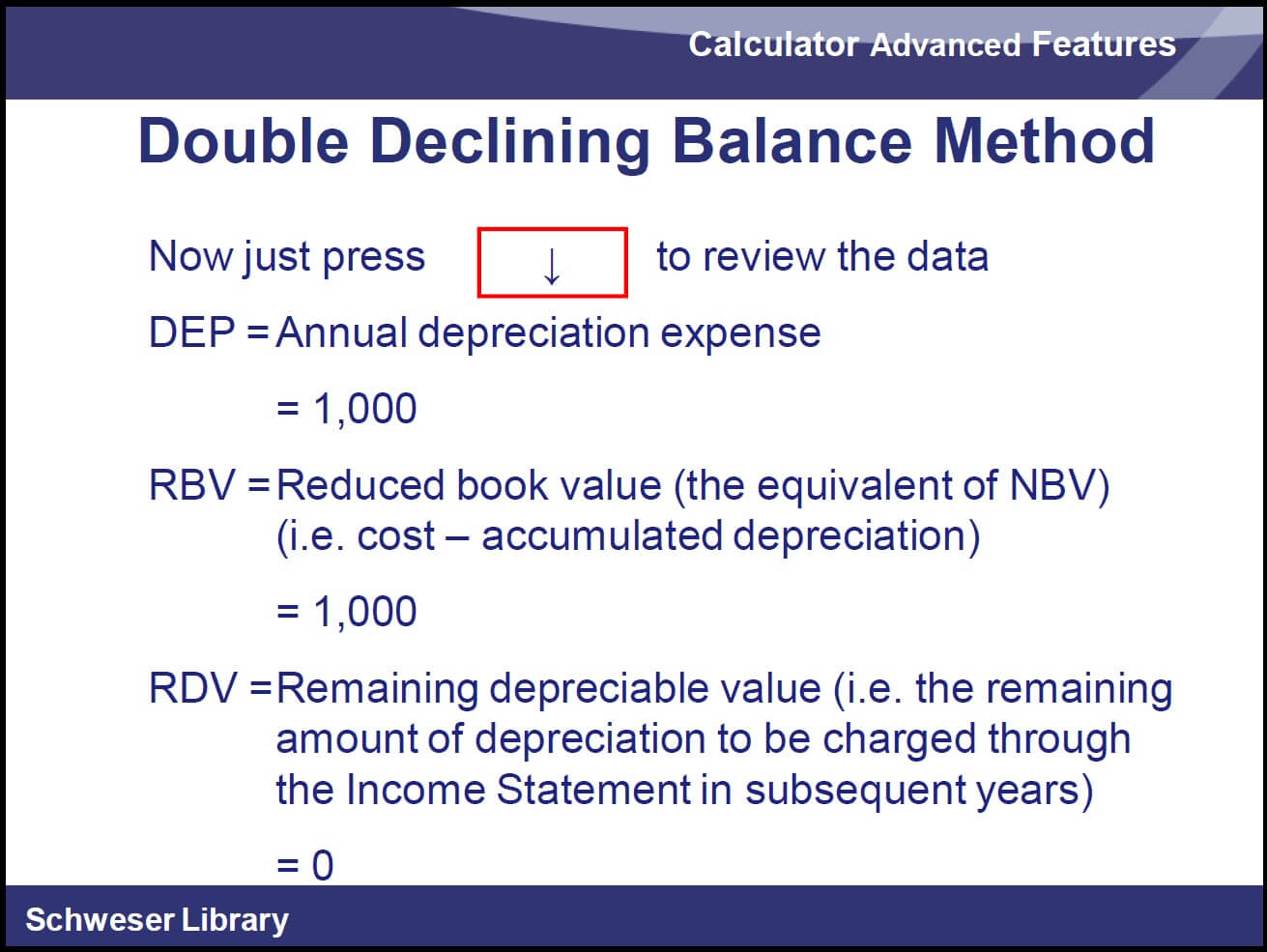
And now we can just review the data. Annual depreciation in that second year is 1,000. Reduced book value, at its cost minus accumulated depreciation, is 1,000 at the end of the second year. Remaining depreciable amount, nothing.
Essentially, we’ve taken 2,000 the first year, which was two-fourths times the 4,000. One-fourth because it’s got four years, two-fourth because we’re using Double Declining Balance. And because we’re using Double Declining Balance, we multiply it times the beginning book value, not times the difference between cost and salvage value. So, the remaining depreciation after the two years of Double Declining Balance is zero.
That’s a lot of the functions between the video volume on the basic functions and this one on the advanced functions, or uses of the TI calculator. So, hopefully, this will give you all the tools you need to make this your new best friend for dealing with problems in finance, corporate finance, debt securities, IRR, NPV, and all of that.
Try Some Free CFA Exam Sample Questions
Looking for Additional CFA Exam Instruction?
Choose from Kaplan Schweser’s CFA exam study materials available for all CFA Program levels.
Take a free diagnostic exam
Feeling Ready For The Exam?

Free eBook: Before You Decide to Sit for the CFA® Program Exam

Free eBook: CFAS® Program Fundamentals, 2nd Edition
Ready to Pass the CFA® Exam?


